Sequence Transition Rate Plot — ggseqtrplot • ggseqplot

Function for plotting transition rate matrix of sequence states internally computed by TraMineR::seqtrate (Gabadinho et al. 2011) . Plot is generated using ggplot2 (Wickham 2016) .

Usage

ggseqtrplot(
  seqdata,
  dss = TRUE,
  group = NULL,
  no.n = FALSE,
  weighted = TRUE,
  with.missing = FALSE,
  labsize = NULL,
  axislabs = "labels",
  x_n.dodge = 1,
  facet_ncol = NULL,
  facet_nrow = NULL
)

Arguments

seqdata: State sequence object (class stslist) created with the TraMineR::seqdef function.
dss: specifies if transition rates are computed for STS or DSS (default) sequences
group: A vector of the same length as the sequence data indicating group membership. When not NULL, a distinct plot is generated for each level of group.
no.n: specifies if number of (weighted) sequences is shown in grouped (faceted) graph
weighted: Controls if weights (specified in TraMineR::seqdef) should be used. Default is TRUE, i.e. if available weights are used
with.missing: Specifies if missing state should be considered when computing the transition rates (default is FALSE).
labsize: Specifies the font size of the labels within the tiles (if not specified ggplot2's default is used)
axislabs: specifies if sequence object's long "labels" (default) or the state names from its "alphabet" attribute should be used.
x_n.dodge: allows to print the labels of the x-axis in multiple rows to avoid overlapping.
facet_ncol: Number of columns in faceted (i.e. grouped) plot
facet_nrow: Number of rows in faceted (i.e. grouped) plot

Value

A tile plot of transition rates.

Details

The transition rates are obtained by an internal call of TraMineR::seqtrate. This requires that the input data (seqdata) are stored as state sequence object (class stslist) created with the TraMineR::seqdef function. As STS based transition rates tend to be dominated by high values on the diagonal, it might be worthwhile to examine DSS sequences instead (dss = TRUE)). In this case the resulting plot shows the transition rates between episodes of distinct states.

In any case (DSS or STS) the transitions rates are reshaped into a a long data format to enable plotting with ggplot2. The resulting output then is prepared to be plotted with ggplot2::geom_tile. The data and specifications used for rendering the plot can be obtained by storing the plot as an object. The appearance of the plot can be adjusted just like with every other ggplot (e.g., by changing the theme or the scale using + and the respective functions).

References

Gabadinho A, Ritschard G, Müller NS, Studer M (2011). “Analyzing and Visualizing State Sequences in R with TraMineR.” Journal of Statistical Software, 40(4), 1--37. doi:10.18637/jss.v040.i04 .

Wickham H (2016). ggplot2: Elegant Graphics for Data Analysis, Use R!, 2nd ed. edition. Springer, Cham. doi:10.1007/978-3-319-24277-4 .

Author

Marcel Raab

Examples

# Use example data from TraMineR: biofam data set
data(biofam)

# We use only a sample of 300 cases
set.seed(10)
biofam <- biofam[sample(nrow(biofam),300),]
biofam.lab <- c("Parent", "Left", "Married", "Left+Marr",
                "Child", "Left+Child", "Left+Marr+Child", "Divorced")
biofam.seq <- seqdef(biofam, 10:25, labels=biofam.lab, weights = biofam$wp00tbgs)
#>  [>] 8 distinct states appear in the data: 
#>      1 = 0
#>      2 = 1
#>      3 = 2
#>      4 = 3
#>      5 = 4
#>      6 = 5
#>      7 = 6
#>      8 = 7
#>  [>] state coding:
#>        [alphabet]  [label]  [long label] 
#>      1  0           0        Parent
#>      2  1           1        Left
#>      3  2           2        Married
#>      4  3           3        Left+Marr
#>      5  4           4        Child
#>      6  5           5        Left+Child
#>      7  6           6        Left+Marr+Child
#>      8  7           7        Divorced
#>  [>] sum of weights: 330.07 - min/max: 0/6.02881860733032
#>  [>] 300 sequences in the data set
#>  [>] min/max sequence length: 16/16

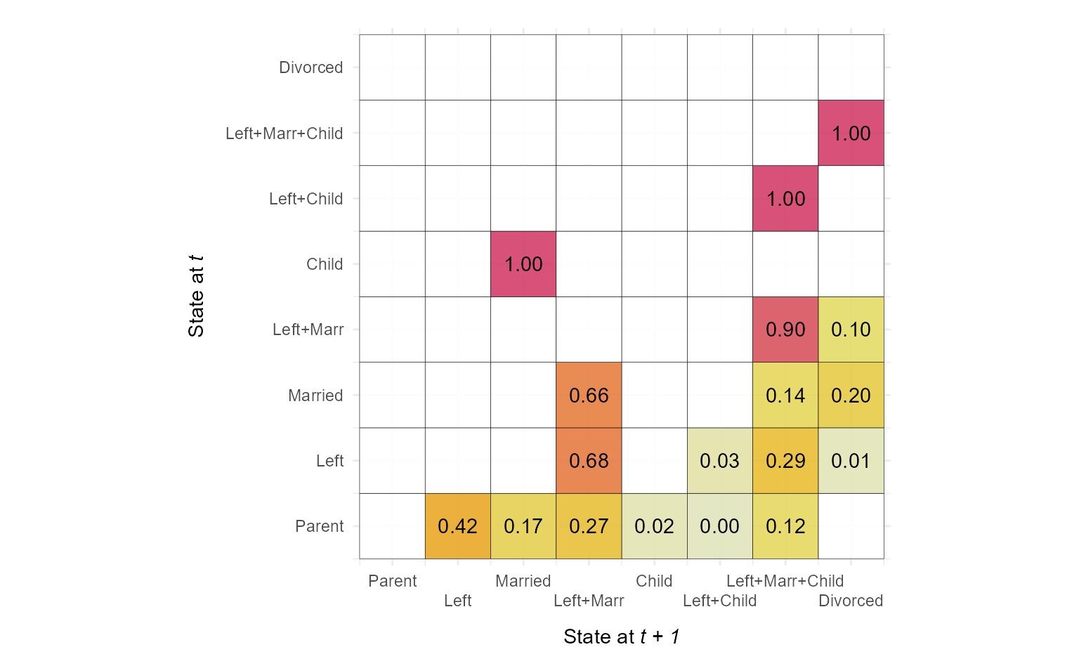
# Basic transition rate plot (with adjusted x-axis labels)
ggseqtrplot(biofam.seq, x_n.dodge = 2)
#>  [>] computing transition probabilities for states 0/1/2/3/4/5/6/7 ...


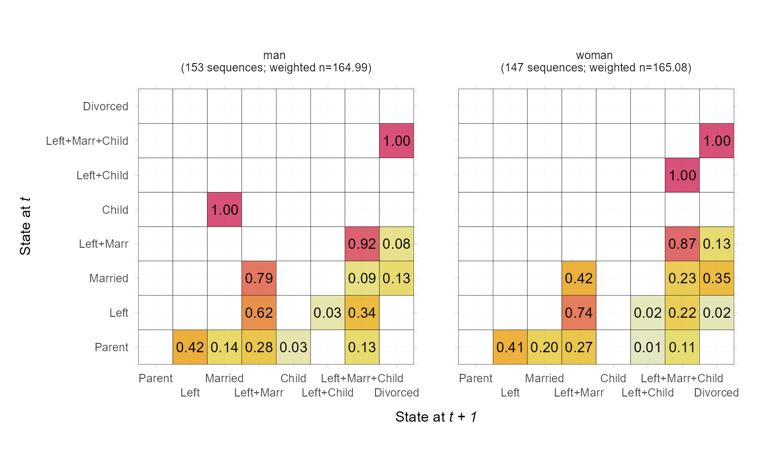
# Transition rate with group variable (with and without weights)
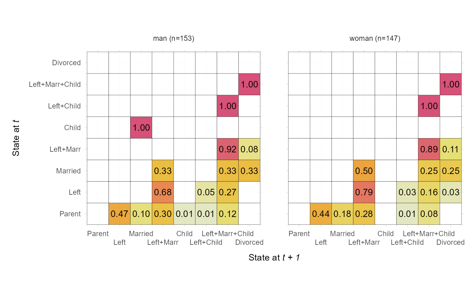
ggseqtrplot(biofam.seq, group=biofam$sex, x_n.dodge = 2)
#>  [>] computing transition probabilities for states 0/1/2/3/4/5/6/7 ...
#>  [>] computing transition probabilities for states 0/1/2/3/4/5/6/7 ...

ggseqtrplot(biofam.seq, group=biofam$sex, x_n.dodge = 2, weighted = FALSE)
#>  [>] computing transition probabilities for states 0/1/2/3/4/5/6/7 ...
#>  [>] computing transition probabilities for states 0/1/2/3/4/5/6/7 ...