Relative Frequency Sequence Plot — ggseqrfplot • ggseqplot

Function for rendering sequence index plots with ggplot2 instead of base R's plot function that is used by TraMineR::seqrfplot. Note that ggseqrfplot uses patchwork to combine the different components of the plot. The function and the documentation draw heavily from TraMineR::seqrf.

Usage

ggseqrfplot(
  seqdata = NULL,
  diss = NULL,
  k = NULL,
  sortv = "mds",
  weighted = TRUE,
  grp.meth = "prop",
  squared = FALSE,
  pow = NULL,
  seqrfobject = NULL,
  border = FALSE,
  ylab = NULL,
  yaxis = TRUE,
  which.plot = "both",
  quality = TRUE,
  box.color = NULL,
  box.fill = NULL,
  box.alpha = NULL,
  outlier.jitter.height = 0,
  outlier.color = NULL,
  outlier.fill = NULL,
  outlier.shape = 19,
  outlier.size = 1.5,
  outlier.stroke = 0.5,
  outlier.alpha = NULL
)

Arguments

seqdata: State sequence object (class stslist) created with the TraMineR::seqdef function. seqdata is ignored if seqrfobject is specified.
diss: pairwise dissimilarities between sequences in seqdata (see TraMineR::seqdist). diss is ignored if seqrfobject is specified.
k: integer specifying the number of frequency groups. When NULL, k is set as the minimum between 100 and the sum of weights over 10. k is ignored if seqrfobject is specified.
sortv: optional sorting vector of length nrow(diss) that may be used to compute the frequency groups. If NULL, the original data order is used. If mds (default), the first MDS factor of diss (diss^2 when squared=TRUE) is used. Ties are randomly ordered. Also allows for the usage of the string inputs: "from.start" or "from.end" (see ggseqiplot). sortv is ignored if seqrfobject is specified.
weighted: Controls if weights (specified in TraMineR::seqdef) should be used. Default is TRUE, i.e. if available weights are used.
grp.meth: Character string. One of "prop", "first", and "random". Grouping method. See details. grp.meth is ignored if seqrfobject is specified.
squared: Logical. Should medoids (and computation of sortv when applicable) be based on squared dissimilarities? (default is FALSE). squared is ignored if seqrfobject is specified.
pow: Dissimilarity power exponent (typically 1 or 2) for computation of pseudo R2 and F. When NULL, pow is set as 1 when squared = FALSE, and as 2 otherwise. pow is ignored if seqrfobject is specified.
seqrfobject: object of class seqrf generated with TraMineR::seqrf. Default is NULL; either seqrfobject or seqdata and diss have to specified
border: if TRUE bars of index plot are plotted with black outline; default is FALSE (also accepts NULL)
ylab: character string specifying title of y-axis. If NULL axis title is "Frequency group"
yaxis: Controls if a y-axis is plotted. When set as TRUE, index of frequency groups is displayed.
which.plot: character string specifying which components of relative frequency sequence plot should be displayed. Default is "both". If set to "medoids" only the index plot of medoids is shown. If "diss.to.med" only the box plots of the group-specific distances to the medoids are shown.
quality: specifies if representation quality is shown as figure caption; default is TRUE
box.color: specifies color of boxplot borders; default is "black
box.fill: specifies fill color of boxplots; default is "white"
box.alpha: specifies alpha value of boxplot fill color; default is 1
outlier.jitter.height: if greater than 0 outliers are jittered vertically. If greater than .375 height is automatically adjusted to be aligned with the box width.
outlier.color, outlier.fill, outlier.shape, outlier.size, outlier.stroke, outlier.alpha: parameters to change the appearance of the outliers. Uses defaults of ggplot2::geom_boxplot

Value

A relative frequency sequence plot using ggplot.

Details

This function renders relative frequency sequence plots using either an internal call of TraMineR::seqrf or by using an object of class "seqrf" generated with TraMineR::seqrf.

For further details on the technicalities we refer to the excellent documentation of TraMineR::seqrf. A detailed account of relative frequency index plot can be found in the original contribution by Fasang and Liao (2014) .

ggseqrfplot renders the medoid sequences extracted by TraMineR::seqrf with an internal call of ggseqiplot. For the box plot depicting the distances to the medoids ggseqrfplot uses geom_boxplot and geom_jitter. The latter is used for plotting the outliers.

Note that ggseqrfplot renders in the box plots analogous to the those produced by TraMineR::seqrfplot. Actually, the box plots produced with TraMineR::seqrfplot and ggplot2::geom_boxplot might slightly differ due to differences in the underlying computations of grDevices::boxplot.stats and ggplot2::stat_boxplot.

Note that ggseqrfplot uses patchwork to combine the different components of the plot. If you want to adjust the appearance of the composed plot, for instance by changing the plot theme, you should consult the documentation material of patchwork.

At this point ggseqrfplot does not support a grouping option. For plotting multiple groups, I recommend to produce group specific seqrfobjects or plots and to arrange them in a common plot using patchwork. See Example 6 in the vignette for further details: vignette("ggseqplot", package = "ggseqplot")

References

Fasang AE, Liao TF (2014). “Visualizing Sequences in the Social Sciences: Relative Frequency Sequence Plots.” Sociological Methods & Research, 43(4), 643–676. doi:10.1177/0049124113506563 .

Author

Marcel Raab

Examples

library(TraMineR)
library(ggplot2)
library(patchwork)

# From TraMineR::seqprf
# Defining a sequence object with the data in columns 10 to 25
# (family status from age 15 to 30) in the biofam data set
data(biofam)
biofam.lab <- c("Parent", "Left", "Married", "Left+Marr",
  "Child", "Left+Child", "Left+Marr+Child", "Divorced")

# Here, we use only 100 cases selected such that all elements
# of the alphabet be present.
# (More cases and a larger k would be necessary to get a meaningful example.)
biofam.seq <- seqdef(biofam[501:600, 10:25], labels=biofam.lab,
                     weights=biofam[501:600,"wp00tbgs"])
#>  [>] 8 distinct states appear in the data: 
#>      1 = 0
#>      2 = 1
#>      3 = 2
#>      4 = 3
#>      5 = 4
#>      6 = 5
#>      7 = 6
#>      8 = 7
#>  [>] state coding:
#>        [alphabet]  [label]  [long label] 
#>      1  0           0        Parent
#>      2  1           1        Left
#>      3  2           2        Married
#>      4  3           3        Left+Marr
#>      5  4           4        Child
#>      6  5           5        Left+Child
#>      7  6           6        Left+Marr+Child
#>      8  7           7        Divorced
#>  [>] sum of weights: 111.62 - min/max: 0/4.17260217666626
#>  [>] 100 sequences in the data set
#>  [>] min/max sequence length: 16/16
diss <- seqdist(biofam.seq, method = "LCS")
#>  [>] 100 sequences with 8 distinct states
#>  [>] creating a 'sm' with a substitution cost of 2
#>  [>] creating 8x8 substitution-cost matrix using 2 as constant value
#>  [>] 76 distinct  sequences 
#>  [>] min/max sequence lengths: 16/16
#>  [>] computing distances using the LCS metric
#>  [>] elapsed time: 0.017 secs


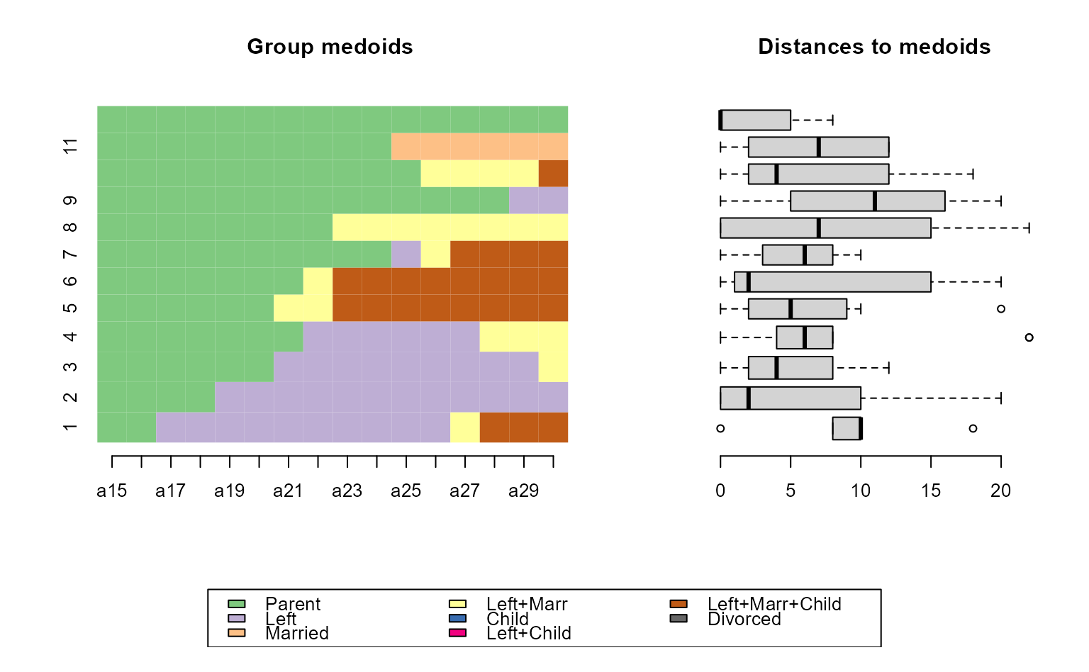
# Using 12 groups and default MDS sorting
# and original method by Fasang and Liao (2014)

# ... with TraMineR::seqrfplot (weights have to be turned off)
seqrfplot(biofam.seq, weighted = FALSE, diss = diss, k = 12,
          grp.meth="first", which.plot = "both")
#>  [>] Using k=12 frequency groups with grp.meth='first'
#>  [>] Pseudo/medoid-based-R2: 0.4620155
#>  [>] Pseudo/medoid-based-F statistic: 6.870317, p-value: 3.09994e-08


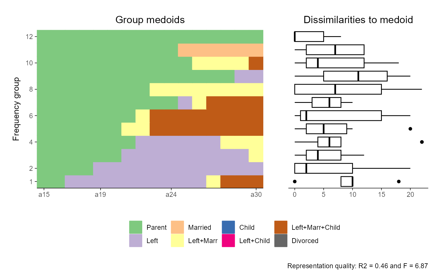
# ... with ggseqrfplot
ggseqrfplot(biofam.seq, weighted = FALSE, diss = diss, k = 12, grp.meth="first")
#>  [>] Using k=12 frequency groups with grp.meth='first'
#>  [>] Pseudo/medoid-based-R2: 0.4620155
#>  [>] Pseudo/medoid-based-F statistic: 6.870317, p-value: 3.09994e-08


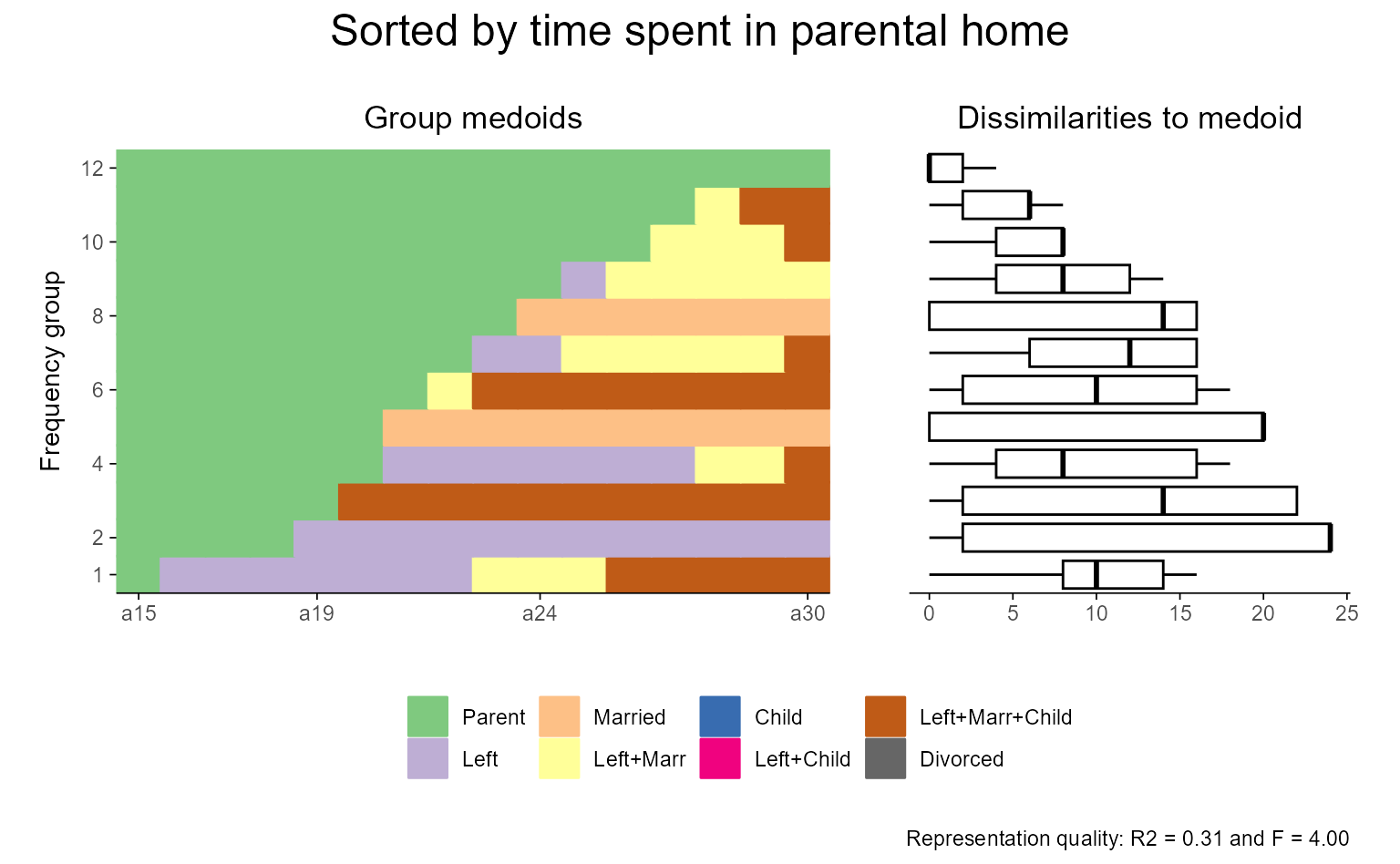
# Arrange sequences by a user specified sorting variable:
# time spent in parental home; has ties
parentTime <- seqistatd(biofam.seq)[, 1]
#>  [>] computing state distribution for 100 sequences ...
b.srf <- seqrf(biofam.seq, diss=diss, k=12, sortv=parentTime)
#>  [>] Using k=12 frequency groups with grp.meth='prop'
#>  [>] Pseudo/medoid-based-R2: 0.3064171
#>  [>] Pseudo/medoid-based-F statistic: 4.001018, p-value: 7.736543e-05
# ... with ggseqrfplot (and some extra annotation using patchwork)
ggseqrfplot(seqrfobject = b.srf) +
  plot_annotation(title = "Sorted by time spent in parental home",
                  theme = theme(plot.title = element_text(hjust = 0.5, size = 18)))