Modal State Sequence Plot — ggseqmsplot • ggseqplot

Function for rendering modal state sequence plot with ggplot2 wickham2016ggseqplot instead of base R's plot function that is used by TraMineR::seqplot gabadinho2011ggseqplot.

Usage

ggseqmsplot(
  seqdata,
  no.n = FALSE,
  barwidth = NULL,
  group = NULL,
  weighted = TRUE,
  with.missing = FALSE,
  border = FALSE,
  facet_ncol = NULL,
  facet_nrow = NULL
)

Arguments

seqdata: State sequence object (class stslist) created with the TraMineR::seqdef function.
no.n: specifies if number of (weighted) sequences is shown (default is TRUE)
barwidth: specifies width of bars (default is NULL); valid range: (0, 1]
group: A vector of the same length as the sequence data indicating group membership. When not NULL, a distinct plot is generated for each level of group.
weighted: Controls if weights (specified in TraMineR::seqdef) should be used. Default is TRUE, i.e. if available weights are used
with.missing: Specifies if missing states should be considered when computing the state distributions (default is FALSE).
border: if TRUE bars are plotted with black outline; default is FALSE (also accepts NULL)
facet_ncol: Number of columns in faceted (i.e. grouped) plot
facet_nrow: Number of rows in faceted (i.e. grouped) plot

Value

A modal state sequence plot. If stored as object the resulting list object also contains the data (long format) used for rendering the plot

Details

The function uses TraMineR::seqmodst to obtain the modal states and their prevalence. This requires that the input data (seqdata) are stored as state sequence object (class stslist) created with the TraMineR::seqdef function.

The data on the modal states and their prevalences are reshaped to be plotted with ggplot2::geom_bar. The data and specifications used for rendering the plot can be obtained by storing the plot as an object. The appearance of the plot can be adjusted just like with every other ggplot (e.g., by changing the theme or the scale using + and the respective functions).

References

Author

Marcel Raab

Examples

# Use example data from TraMineR: actcal data set
data(actcal)

# We use only a sample of 300 cases
set.seed(1)
actcal <- actcal[sample(nrow(actcal), 300), ]
actcal.lab <- c("> 37 hours", "19-36 hours", "1-18 hours", "no work")
actcal.seq <- seqdef(actcal, 13:24, labels = actcal.lab)
#>  [>] 4 distinct states appear in the data: 
#>      1 = A
#>      2 = B
#>      3 = C
#>      4 = D
#>  [>] state coding:
#>        [alphabet]  [label]  [long label] 
#>      1  A           A        > 37 hours
#>      2  B           B        19-36 hours
#>      3  C           C        1-18 hours
#>      4  D           D        no work
#>  [>] 300 sequences in the data set
#>  [>] min/max sequence length: 12/12

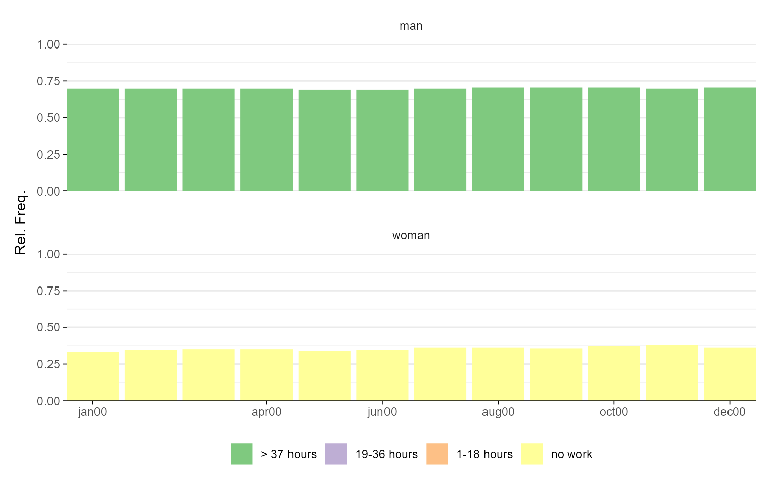
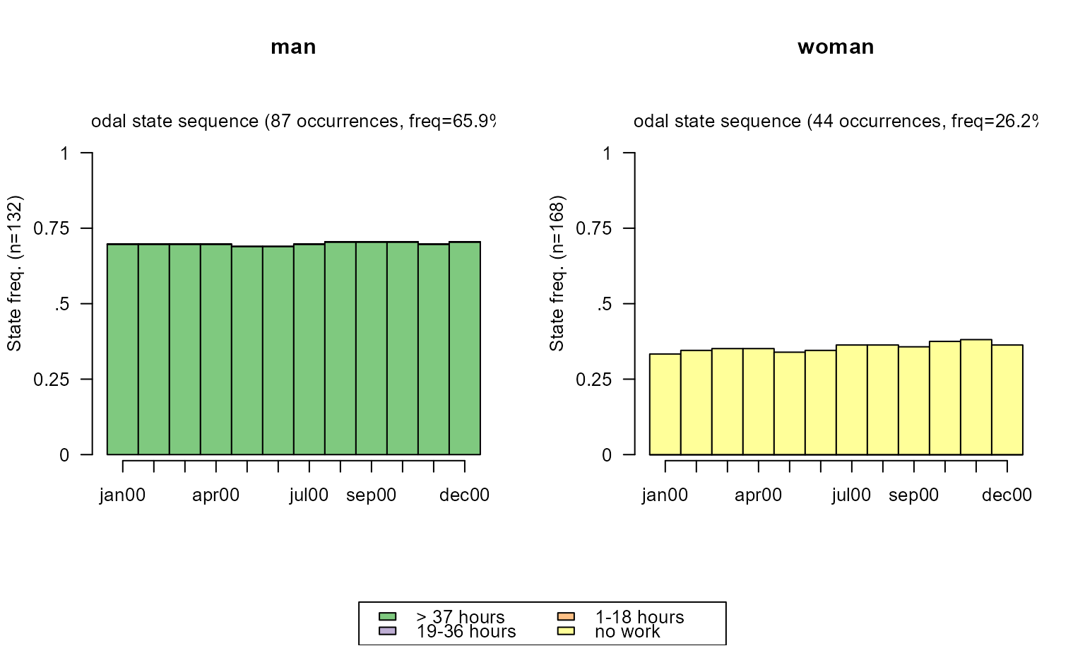
# modal state sequence plot; grouped by sex
# with TraMineR::seqplot
seqmsplot(actcal.seq, group = actcal$sex)

# with ggseqplot
ggseqmsplot(actcal.seq, group = actcal$sex)

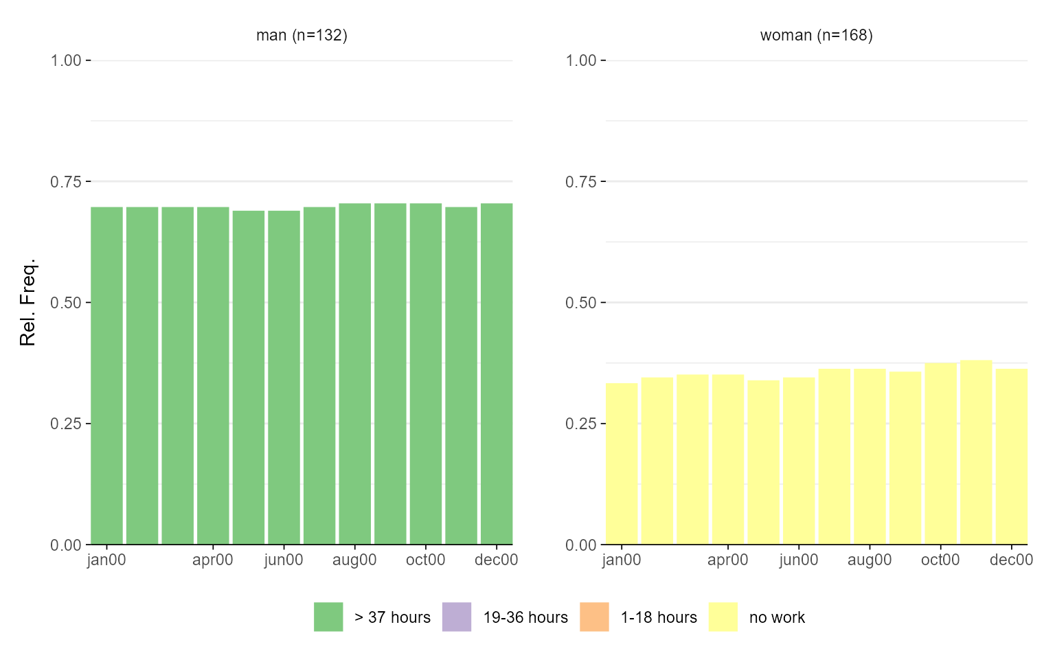# with ggseqplot and some layout changes
ggseqmsplot(actcal.seq, group = actcal$sex, no.n = TRUE, border = FALSE, facet_nrow = 2)