Sequence Frequency Plot

Function for rendering sequence index plot of the most frequent sequences of a state sequence object using ggplot2 (Wickham 2016) instead of base R's plot function that is used by TraMineR::seqplot / TraMineR::plot.stslist.freq (Gabadinho et al. 2011) .

Usage

ggseqfplot(
  seqdata,
  group = NULL,
  ranks = 1:10,
  weighted = TRUE,
  border = FALSE,
  proportional = TRUE,
  ylabs = "total",
  no.coverage = FALSE,
  facet_ncol = NULL,
  facet_nrow = NULL
)

Arguments

seqdata: State sequence object (class stslist) created with the TraMineR::seqdef function.
group: A vector of the same length as the sequence data indicating group membership. When not NULL, a distinct plot is generated for each level of group.
ranks: specifies which of the most frequent sequences should be plotted; default is the first ten (1:10); if set to 0 all sequences are displayed
weighted: Controls if weights (specified in TraMineR::seqdef) should be used. Default is TRUE, i.e. if available weights are used
border: if TRUE bars are plotted with black outline; default is FALSE (also accepts NULL)
proportional: if TRUE (default), the sequence heights are displayed proportional to their frequencies
ylabs: defines appearance of y-axis labels; default ("total") only labels min and max (i.e. cumulative relative frequency); if "share" labels indicate relative frequency of each displayed sequence (note: overlapping labels are removed)
no.coverage: specifies if information on total coverage is shown as caption or as part of the group/facet label if ylabs == "share" (default is TRUE)
facet_ncol: Number of columns in faceted (i.e. grouped) plot
facet_nrow: Number of rows in faceted (i.e. grouped) plot

Value

A sequence frequency plot created by using ggplot2. If stored as object the resulting list object (of class gg and ggplot) also contains the data used for rendering the plot.

Details

The subset of displayed sequences is obtained by an internal call of TraMineR::seqtab. The extracted sequences are plotted by a call of ggseqiplot which uses ggplot2::geom_rect to render the sequences. The data and specifications used for rendering the plot can be obtained by storing the plot as an object. The appearance of the plot can be adjusted just like with every other ggplot (e.g., by changing the theme or the scale using + and the respective functions).

Experienced ggplot2 users might notice the customized labeling of the y-axes in the faceted plots (i.e. plots with specified group argument). This has been achieved by utilizing the very helpful ggh4x library.

References

Gabadinho A, Ritschard G, Müller NS, Studer M (2011). “Analyzing and Visualizing State Sequences in R with TraMineR.” Journal of Statistical Software, 40(4), 1--37. doi:10.18637/jss.v040.i04 .

Wickham H (2016). ggplot2: Elegant Graphics for Data Analysis, Use R!, 2nd ed. edition. Springer, Cham. doi:10.1007/978-3-319-24277-4 .

Author

Marcel Raab

Examples

# Use example data from TraMineR: actcal data set
data(actcal)

# We use only a sample of 300 cases
set.seed(1)
actcal <- actcal[sample(nrow(actcal), 300), ]
actcal.lab <- c("> 37 hours", "19-36 hours", "1-18 hours", "no work")
actcal.seq <- seqdef(actcal, 13:24, labels = actcal.lab)
#>  [>] 4 distinct states appear in the data: 
#>      1 = A
#>      2 = B
#>      3 = C
#>      4 = D
#>  [>] state coding:
#>        [alphabet]  [label]  [long label] 
#>      1  A           A        > 37 hours
#>      2  B           B        19-36 hours
#>      3  C           C        1-18 hours
#>      4  D           D        no work
#>  [>] 300 sequences in the data set
#>  [>] min/max sequence length: 12/12

# sequence frequency plot
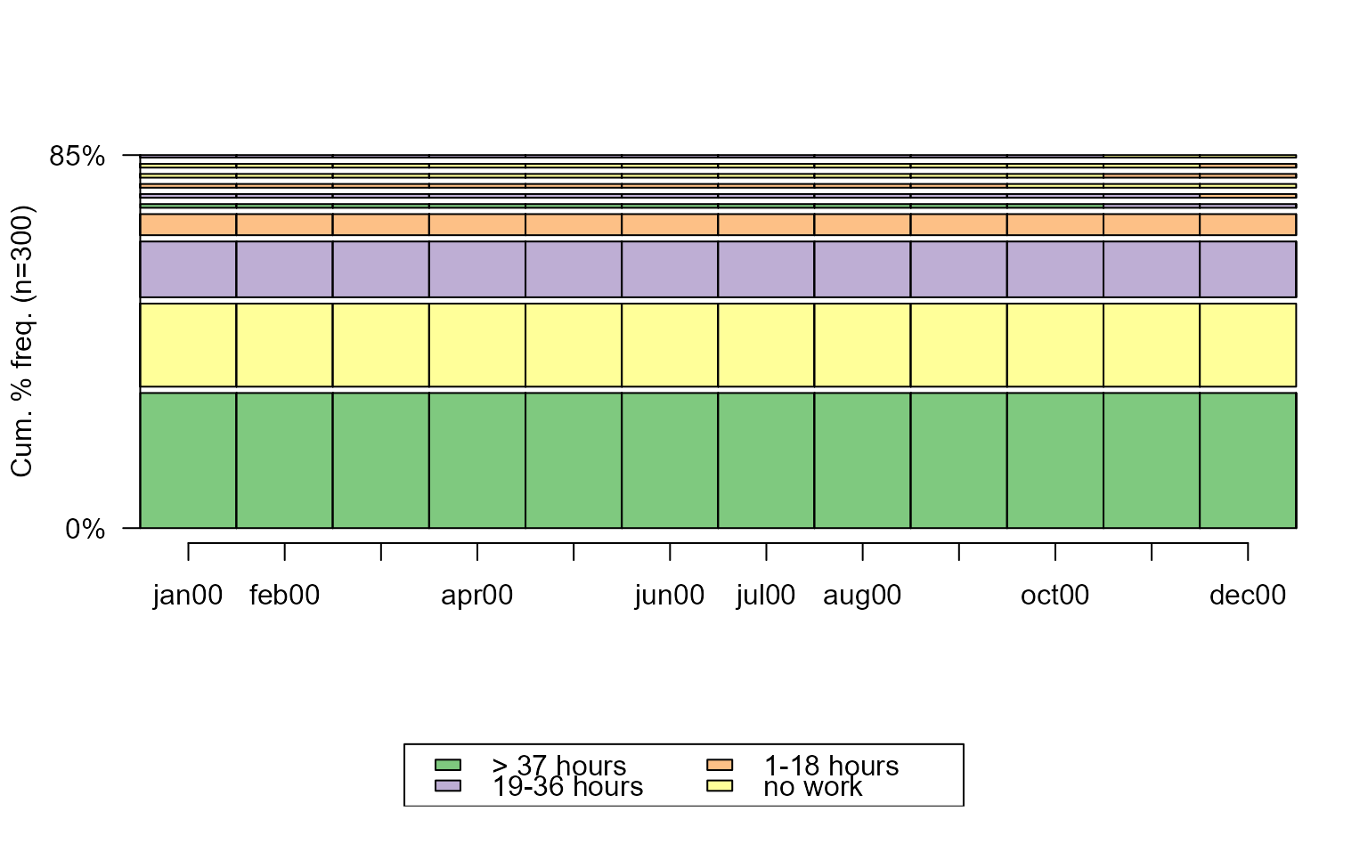
# with TraMineR::seqplot
seqfplot(actcal.seq)

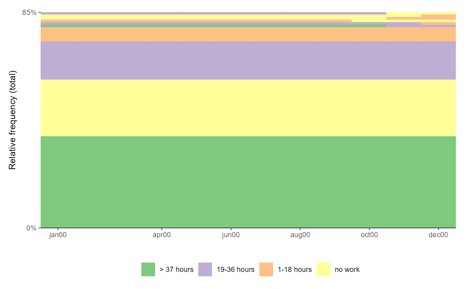
# with ggseqplot
ggseqfplot(actcal.seq)

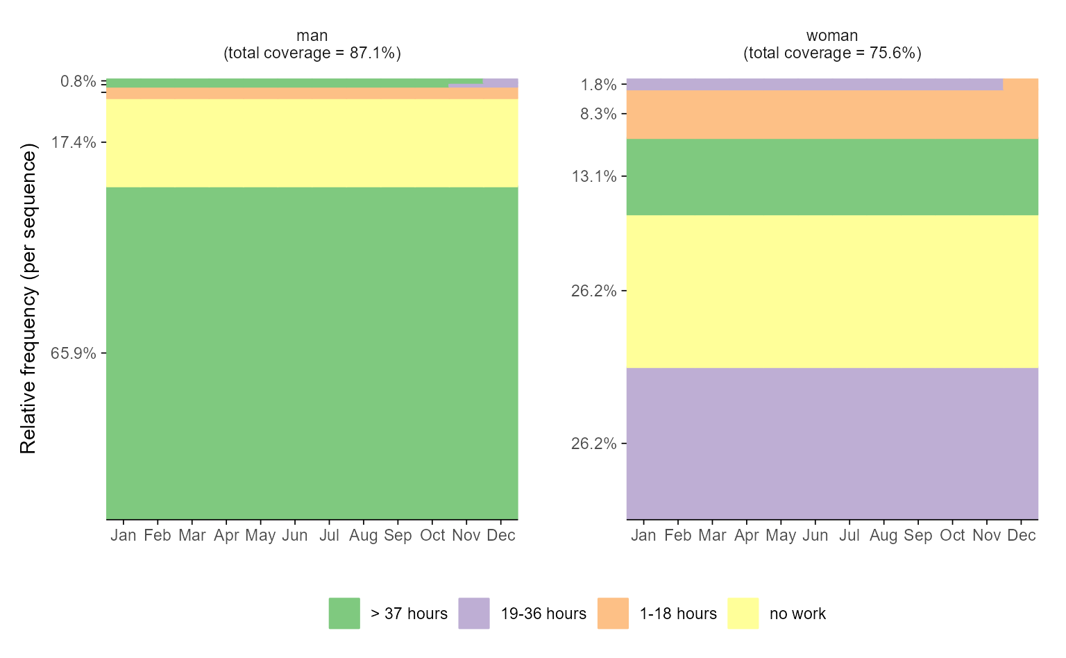
# with ggseqplot applying additional arguments and some layout changes
ggseqfplot(actcal.seq,
           group = actcal$sex,
           ranks = 1:5,
           ylabs = "share") +
  scale_x_discrete(breaks = 1:12,
                   labels = month.abb,
                   expand = expansion(add = c(0.2, 0)))
#> Scale for x is already present.
#> Adding another scale for x, which will replace the existing scale.